When an ML Improvement Doesn’t Survive Validation

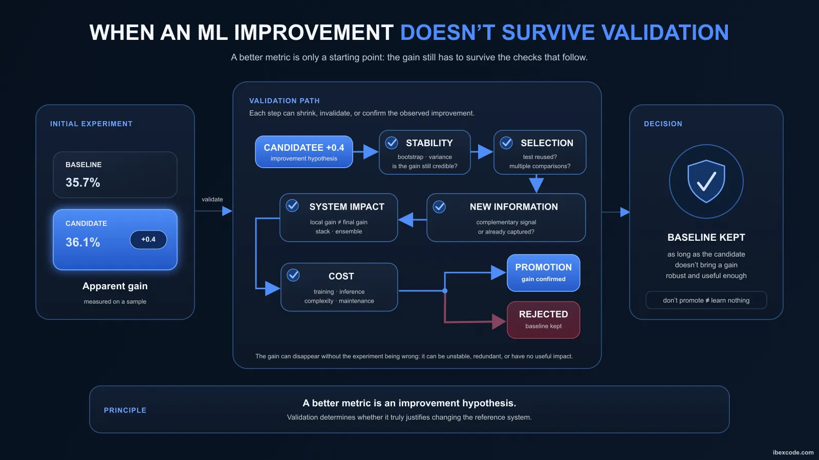
In Machine Learning, getting a better metric is relatively easy.

Getting an improvement that survives more rigorous validation is much harder.

A new feature, a different architecture, or a new model combination can produce an encouraging result in a first experiment:

Baseline      : 35.7%
Candidate     : 36.1%
Gap           : +0.4 point

The natural temptation is then to consider the candidate better.

But this measurement only answers a first question:

Did the candidate perform better on this sample?

It doesn’t yet tell us whether the observed gap is stable enough, whether it actually carries additional information, or whether it will hold once the candidate is reintegrated into the full system.

In an already mature ML system, many experiments follow a much less spectacular path:

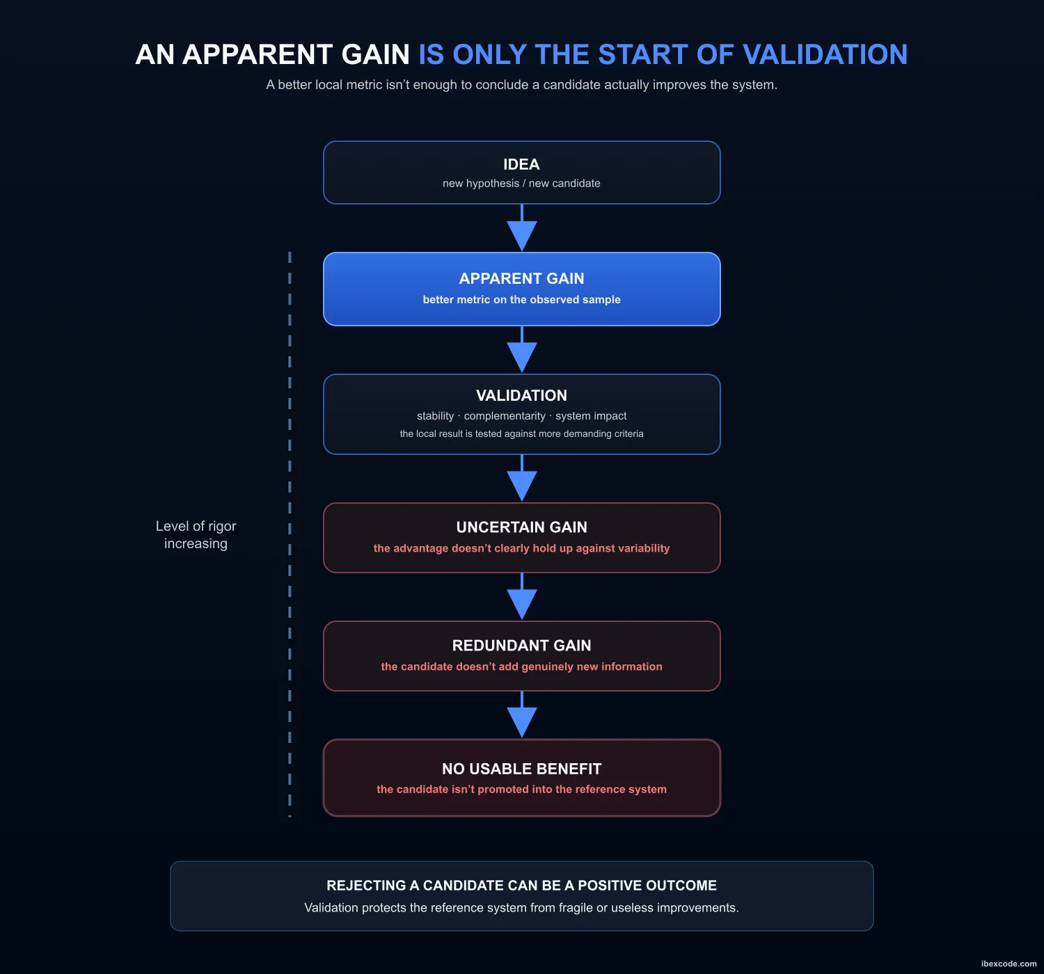
This outcome isn’t necessarily a failed experiment.

Eliminating an improvement that doesn’t survive validation is precisely part of the process that keeps the reference system from degrading.

---

1. A better metric is not yet an improvement

Suppose two models evaluated over exactly the same period:

Model A: 35.7%
Model B: 36.1%

It’s perfectly correct to say that B performs better on this sample.

It’s much harder to say:

B is a better model.

Between these two statements lies the entire question of validation.

A metric is computed over a finite set of observations. Its value therefore partly depends on the examples present in that set.

When the differences between models are large, this variability rarely changes the conclusion.

But as a system improves, gains generally get smaller.

The most obvious errors have already been fixed, the most informative features are already in place, and several model families have often already been explored.

Eventually you end up comparing candidates separated by a few tenths of a point.

At that scale, evaluation variability can become comparable to the gain being sought.

A gap of +0.4 point should therefore be treated as an observation to test, not immediately as a property of the new model.

---

2. Measuring the uncertainty around a gain

When two models are evaluated on the same events, the important information isn’t only in their final metrics.

It’s also in how their results differ on the same observations.

A particularly hard event can degrade both models at once. What matters to us isn’t just how hard it is, but whether one of the two systems handles it better than the other.

For each event i, we can consider the difference:

Δᵢ = result_B(i) - result_A(i)

This paired comparison lets us study the candidate’s advantage over the baseline directly.

One way to measure its stability is then to use a paired bootstrap.

The idea is to resample the evaluation events with replacement. For each resulting sample, both models’ performance is recomputed on exactly the same events, and the difference is measured:

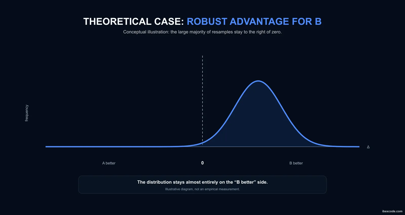
Δ = metric(B) - metric(A)

Instead of a single value, we now get a distribution of gains.

If this distribution remains mostly above zero, the resampled datasets generally support the same conclusion.

If it largely crosses zero, the result becomes much more dependent on the sample’s composition: some variants favor the candidate, others lead to a near tie, or even give the advantage to the baseline.

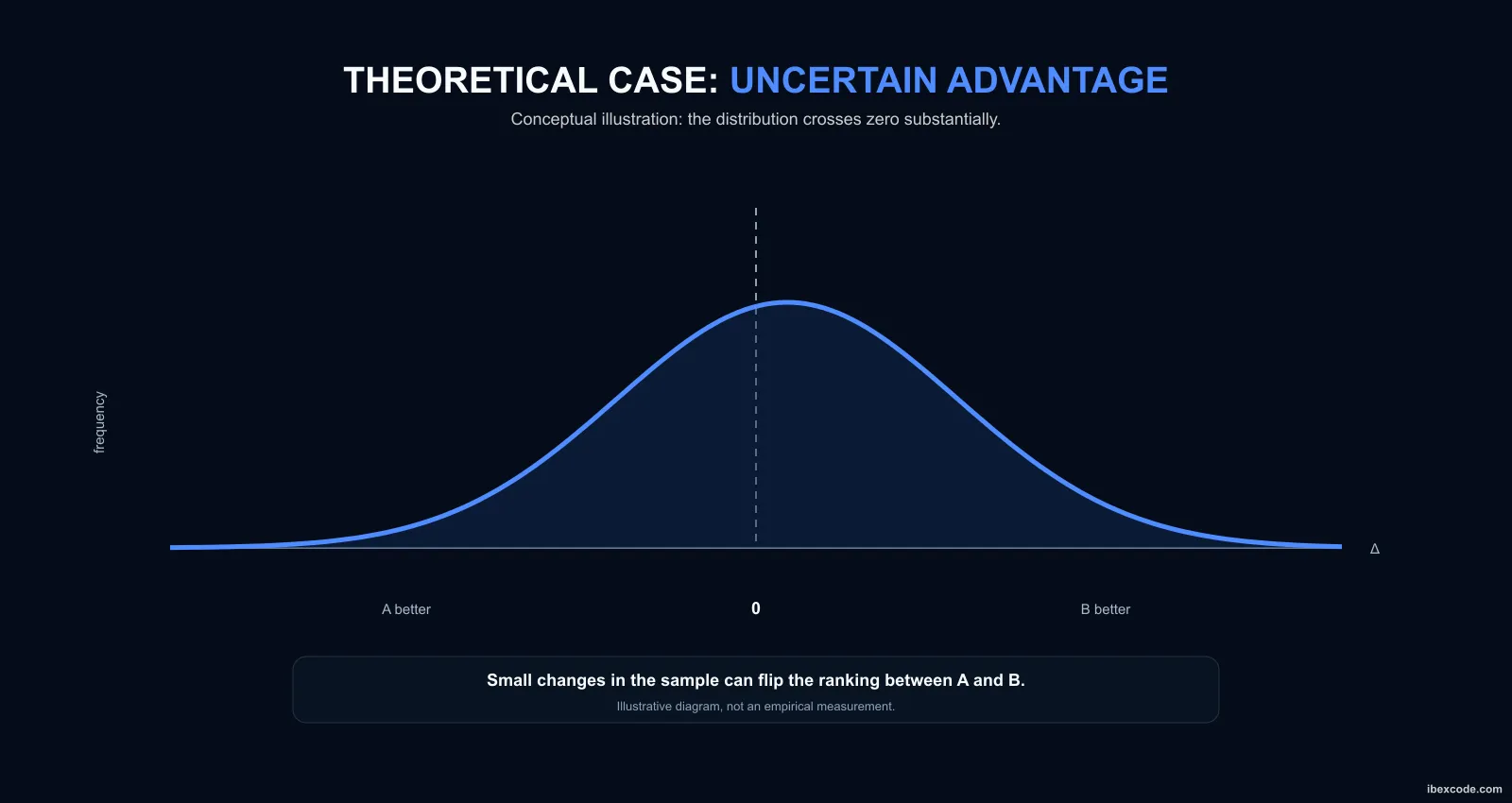
The initial result isn’t wrong.

It’s its interpretation as a sufficiently stable improvement that becomes uncertain.

The distinction matters: noting that B got a better score doesn’t yet mean the available data is enough to establish, with sufficient robustness, that it is actually better.

---

3. The research process itself can bias selection

Another problem appears when the same evaluation set is used repeatedly to guide experiments.

After each trial, the result naturally influences what comes next:

• keep or drop a feature;
• abandon an architecture;
• tweak certain hyperparameters;
• explore a combination that looks promising.

No test-set observation is necessarily injected into training.

Yet, over the course of experiments, the decisions made increasingly depend on results observed on that set.

Suppose, for example, a sequence of experiments:

experiment 01 → no gain
experiment 02 → slight improvement
experiment 03 → degradation
experiment 04 → improvement

The result of experiment 04 can no longer be treated as fully independent of the experimental process that led to it if experiments 02 and 03 influenced what was tested next.

The experimental process itself has gradually used the evaluation set as a source of information.

This phenomenon is different from classic data leakage.

The model didn’t directly learn from the test data.

It’s the research that gradually adapted to the particularities of that set.

The more this loop repeats, the less that set can be considered a fully independent measurement of the decisions that led to the final candidate.

A strict separation between data used to guide research and data reserved for final validation helps limit this problem.

---

4. Running more tests increases the risk of false positives

There’s a second problem, this time statistical, when a campaign involves multiple hypothesis tests.

Suppose we test 100 changes and, in reality, none of them produce an improvement.

Each test still carries some probability of wrongly concluding that an effect exists.

With a significance threshold set at:

α = 0.05

we accept a 5% false-positive risk for a single, isolated test.

But if that same threshold is applied independently to 100 hypotheses, the risk of getting at least one result declared significant by chance becomes much higher.

The results might, for example, look like:

A → not significant
B → not significant
C → not significant
D → significant
E → not significant
...

even though none of the tested changes has a real effect.

The Bonferroni correction is a simple way to control this risk across the whole set of tests.

To keep an overall risk α of 5% across m tests, the individual threshold becomes:

α_test = α / m

For 100 tests:

α_test = 0.05 / 100
       = 0.0005

A result with:

p = 0.01

would be significant under the classic threshold of 0.05, but wouldn’t clear the corrected threshold of 0.0005 here.

Bonferroni is deliberately conservative: while it strongly reduces the risk of false positives, it also makes some real effects harder to detect.

So it isn’t a universal rule to apply mechanically to every ML experimentation campaign.

It does, however, illustrate an important statistical principle: how a test should be interpreted also depends on how many hypotheses are being tested within the family of comparisons you want to control.

This problem is distinct from the selection bias described above.

• In one case, past results progressively influence future experiments.
• In the other, several statistical tests are considered at once, and the false-positive risk that comes from their multiplicity has to be controlled.

Both can naturally show up in the same experimental process, but they aren’t corrected the same way.

---

5. Relevant information can be redundant

An improvement can also disappear for a reason that has nothing to do with statistics: the new information is real, but the system may already capture it in another form.

A new feature can show a measurable relationship with the target without improving the model. Existing variables may already capture all or part of the same information.

Two questions then need to be distinguished:

Does the variable carry information?

and:

Does it provide additional information beyond what the model already captures?

These two questions aren’t equivalent. A feature can be strongly related to the target and still become almost useless once conditioned on the information the model already has.

To improve a mature system, the second question is generally the more important one.

A feature should therefore be judged not only by the signal it contains, but by the additional signal it contributes beyond what the model already captures.

If existing features already capture the same information, a new variable can look relevant when studied on its own while adding no gain once folded into the model.

---

6. A different model doesn’t necessarily produce different errors

The same reasoning applies when a feature is replaced with a new model family.

Two very different algorithms can reach similar performance because they essentially exploit the same information present in the data.

Moving from gradient boosting to a neural network, for example, doesn’t guarantee that the errors actually become different.

This distinction becomes especially important in a model ensemble.

A new candidate that’s slightly weaker on its own can still be interesting if it specifically succeeds on observations where the existing models fail.

Conversely, a candidate that’s slightly better in isolation can add very little to the system if it reproduces almost exactly the same decisions.

The comparison can then focus on:

• Prediction correlation
• Error correlation
• Cases where one model succeeds and the other fails
• Cases uniquely handled correctly by one model
• Impact after combination with the existing models

Similar performance combined with strongly correlated errors and very few unique wins suggests that the architecture change is probably exploiting a large part of the same signal.

Useful diversity cannot be inferred from the choice of algorithm alone. It has to be evaluated through the behaviors actually produced and, ultimately, through its impact on the full system.

---

7. A local gain can disappear in the full system

This question becomes even more important in a multi-level architecture.

Suppose:

L1_A ─┐
      ├──► L2 ─► L3
L1_B ─┘

A new version of L1_A can improve its own metric. But that improvement doesn’t guarantee an improvement in the final output.

The downstream levels already combine several signals. The local gain can therefore be:

• redundant with another model
• already compensated for downstream
• too small to change the final decision
• paired with new errors on other events
• difficult for downstream levels to exploit

So it’s entirely possible for a candidate to beat its baseline at the L1 level without producing any improvement at the full-system level — or even while slightly degrading its final output.

The candidate wasn’t necessarily bad. Its improvement was simply local to a component whose metric isn’t the system’s actual objective.

In a stacking or ensemble architecture, evaluation therefore needs to happen at several levels. The local metric helps understand the component’s behavior.

But the final unit of comparison remains the complete system in which the candidate will actually be used.

---

8. A real gain isn’t necessarily a useful gain

Now suppose the gain survives all the previous checks. One last dimension remains: its cost.

Two candidates can produce exactly the same improvement while having very different operational consequences:

	Candidate A	Candidate B
Gain	+0.3 point	+0.3 point
Change	New feature	New model family
Training	Virtually unchanged	More expensive
Inference	Virtually unchanged	More expensive
Artifacts	Unchanged or limited	Several additional artifacts

On the observed metric, both improvements look equivalent. Operationally, they aren’t.

A change can bring more training time, higher memory usage, slower inference, new dependencies, more artifacts to version, or additional sources of train–serve skew.

The decision is therefore no longer just:

Is the candidate better?

but:

Does the benefit gained justify the added complexity needed to get it?

A statistically credible improvement can thus remain too small to justify changing the reference system.

---

9. Negative experiments still produce useful knowledge

When an experiment doesn’t produce an exploitable gain, it can still narrow the space of plausible hypotheses.

The finding becomes especially interesting when several approaches converge:

new feature       → no robust gain
new model         → similar errors
new architecture  → no system-level gain
new combination   → redundant information

No new model gets promoted.

But several pieces of information have been gained:

• the signal being studied is probably already largely captured
• this direction doesn’t bring the diversity being sought
• nearby variants are less likely to produce a meaningful change
• pursuing this direction is now less likely to be worth the additional effort

The outcome is then no longer simply that an experiment didn’t work.

Several experiments start to indicate that this family of hypotheses adds little new information to the current system.

A negative experiment can therefore produce useful knowledge about the system, even when it produces no new artifact to deploy.

---

10. Knowing when to stop pursuing a direction is part of experimentation

It’s easy to define when to start an experiment. It’s harder to determine when to stop a research direction.

The same idea can produce almost endless new variants: different time windows, transformations, interactions, model families, or combinations. Each one can seem different enough to justify one more test.

But when successive experiments consistently produce small, uncertain gains, similar errors, and no measurable impact on the full system, the likelihood that another nearby variant will materially change the conclusion also decreases. Continuing to explore exactly the same signal then yields diminishing returns.

Stopping a direction doesn’t mean proving it can never produce an improvement. It means, more modestly:

The available results no longer justify allocating more time and compute to this direction over other possible hypotheses.

This decision is itself part of the experimental process. In some cases, the best next step isn’t a new algorithm or a new transformation.

It’s looking for information the current system does not already capture effectively.

---

11. From a better metric to promotion

A candidate improvement can ultimately be evaluated through a sequence of increasingly demanding levels of evidence.

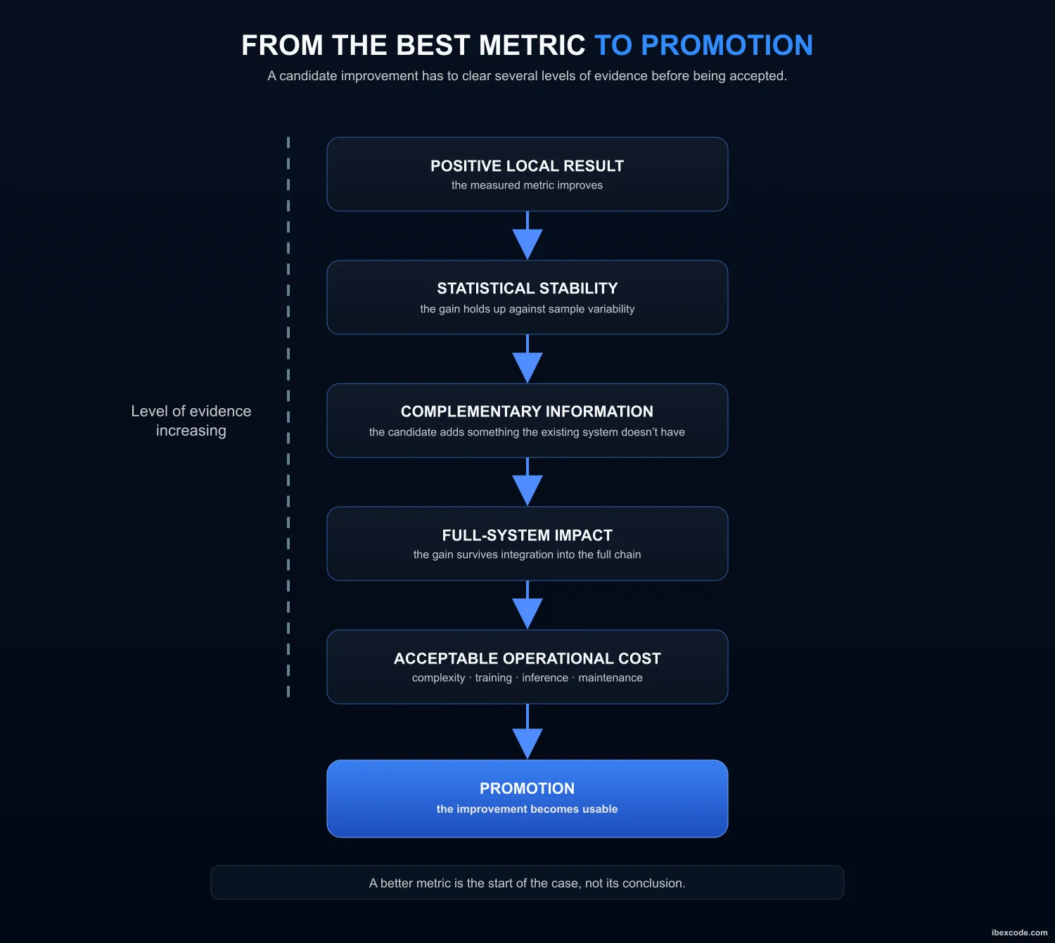
The first positive result, then, isn’t the end of the evaluation.

It’s the start of it.

A candidate can be rejected at any of these stages: too unstable a gain, bias from the selection process, information already captured, errors too similar to those of existing models, no gain on the final system, or disproportionate cost.

Not every change obviously needs the same depth of analysis.

But a general rule emerges:

The smaller the observed gain and the more costly the change, the stronger the evidence needed before promotion.

A better metric is thus an improvement hypothesis. Validation then determines whether that hypothesis actually justifies changing the system.

The initial metric triggers the analysis.

It doesn’t conclude it.

---

12. Conclusion

An improvement observed in a first experiment doesn’t always survive the validations that follow.

The gain can turn out to be too uncertain, partly dependent on the selection process, equivalent to information already captured, or it can simply disappear once the change is folded back into the full system.

This outcome doesn’t make the experiment pointless. On the contrary, it’s exactly what lets you tell apart a gain observed in a particular experiment from an improvement robust enough to change the reference system.

As an ML system matures, this distinction matters more and more. Easy gains become rarer, the gaps between candidates shrink, and a growing share of experiments naturally end up keeping the existing system.

That doesn’t mean research stops moving forward. Establishing that a direction adds no new information, that its gain is too fragile, or that it disappears at the system level also helps clarify what’s actually still left to improve.

The goal, then, isn’t to beat the baseline in every experiment, but to replace it only when an improvement survives validation with enough evidence to justify the change.