Building a Temporal ML Ranking System Without Data Leakage

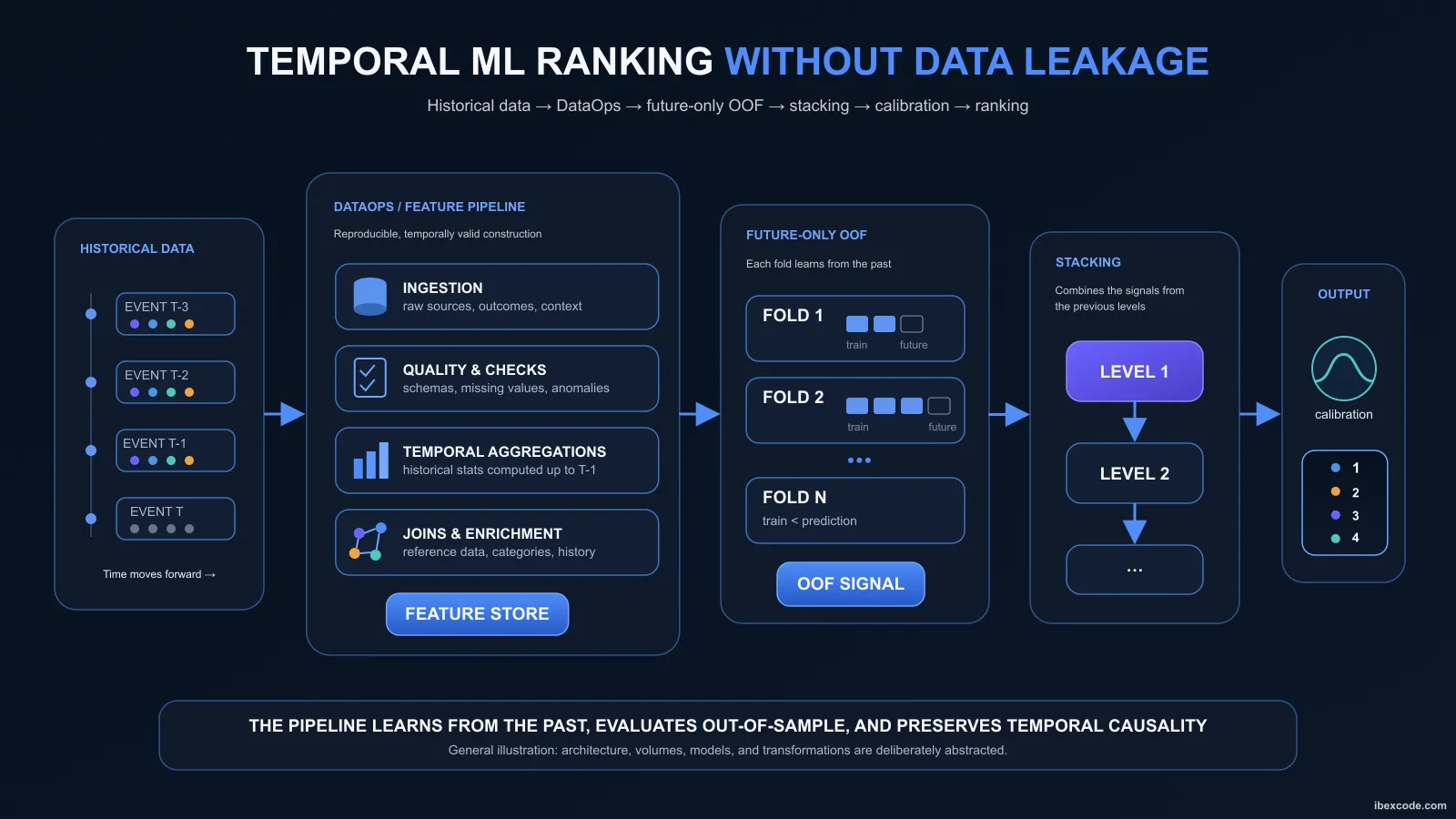
In a Machine Learning system applied to temporal data, a model’s quality can’t be separated from how its training and evaluation data were built.

That constraint becomes more demanding when multiple observations belong to the same event, must be ranked against one another, and predictions from several models are fed into downstream levels of a stack.

The system described here addresses exactly this kind of problem: producing a relative ranking across multiple candidates from historical data, then combining several models within a multi-level architecture.

Its validation rests on one central invariant:

Every historical prediction must be computed using only information that would genuinely have been available at the moment that prediction would have been produced.

Guaranteeing this for a single, isolated model is fairly simple. Maintaining it across feature engineering, several stacking levels, learned transformations, and a calibration stage, however, means treating it as a property of the entire architecture.

---

1. A temporal ranking problem

The dataset is structured around events, each containing multiple candidates.

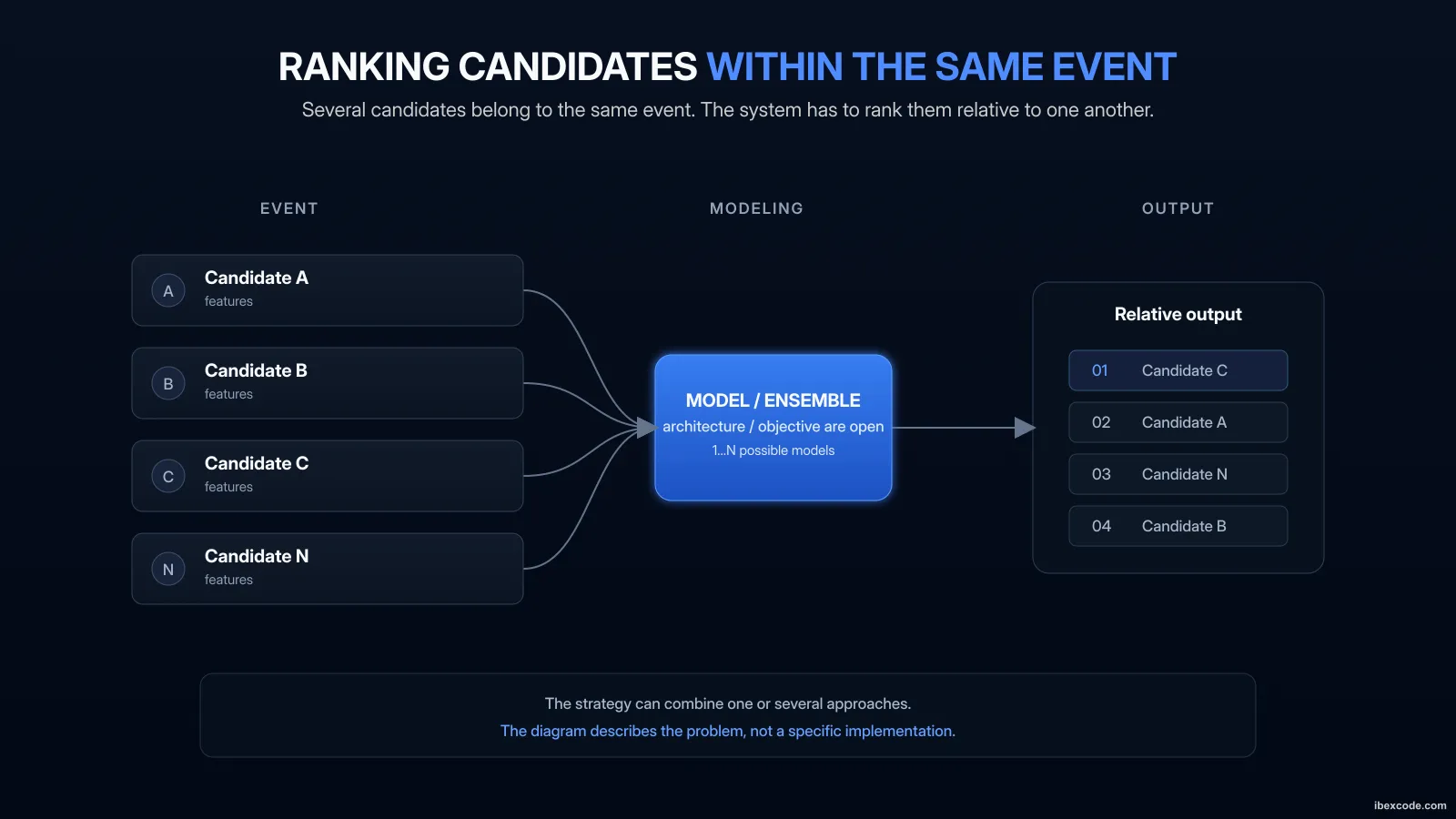
So the system isn’t just trying to estimate a value independently for each observation. It also has to capture the relationships between candidates within each event.

To do this, the architecture can combine several learning objectives or representations of the problem. Some models produce a continuous, per-candidate signal, while others exploit the event’s relative structure more directly.

Different approaches can reach similar overall performance while producing partially different predictions or error patterns. Whether those differences are actually useful can then be evaluated at the downstream levels of the architecture.

Conceptually, one level of the system can be represented like this:

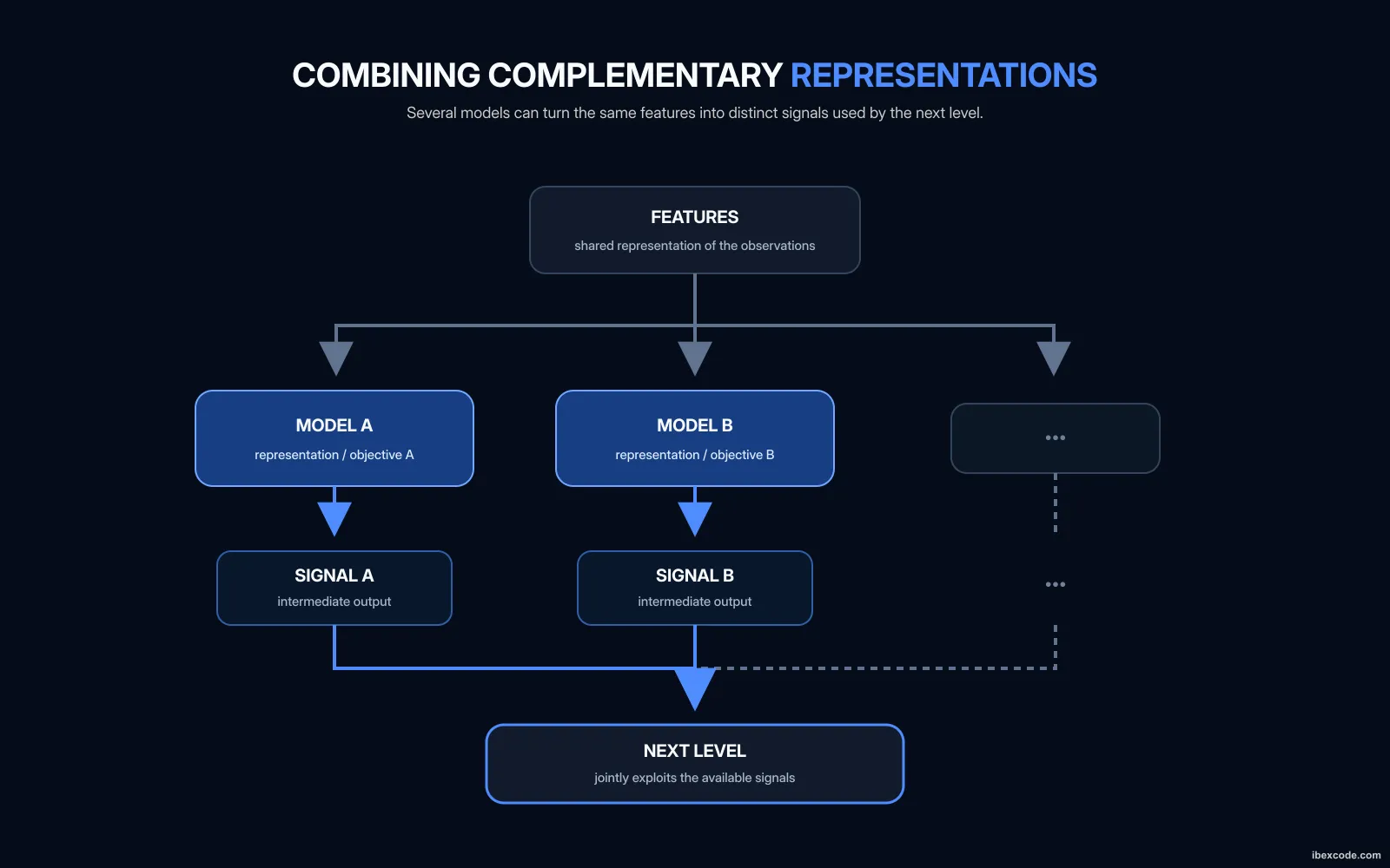
What matters here isn’t exactly which models are used, but how information flows between levels.

This architecture introduces an additional difficulty: the predictions produced by one level can themselves become training data for the next one.

Temporal causality therefore has to be guaranteed not only for the initial dataset, but at every boundary of the stack.

---

2. Temporal causality in the validation protocol

A random split is out of the question.

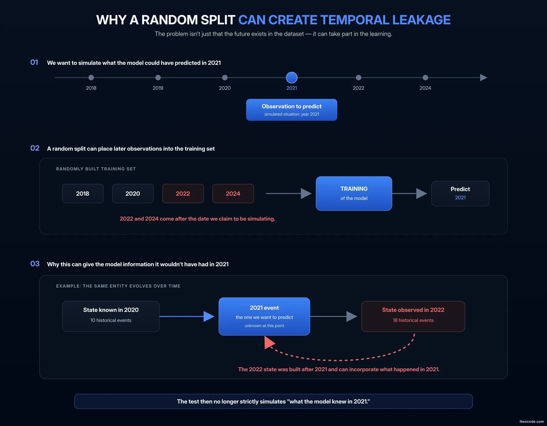
Independence between train and test isn’t enough when a temporal relationship exists. An observation evaluated at time t must be produced by a pipeline whose entire state was built exclusively from information predating t.

This applies to the model, but also to historical aggregations, learned transformations, and every artifact derived from the data.

The fundamental constraint can be written as:

max(train_date) < min(evaluation_date)

The main protocol therefore keeps a strict chronological separation:

TRAIN → CALIBRATION → TEST

The test period stays later than every piece of data used to build the system. This property is enough to evaluate a model trained directly on the training set.

But it’s no longer enough once its predictions are used to train another model.

---

3. Stacking creates a new leakage boundary

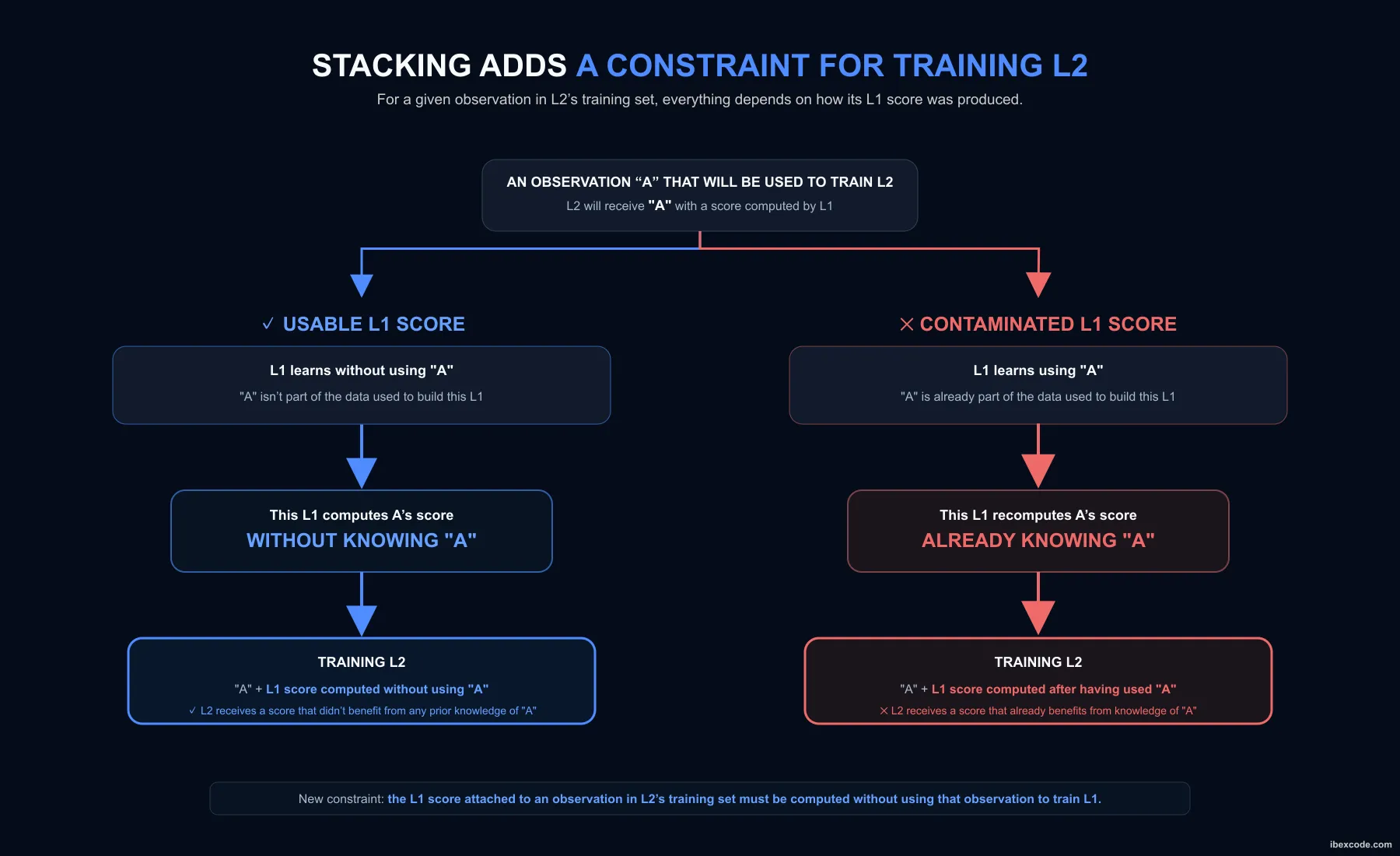
The meta-model has to learn to exploit the outputs of models A and B.

It would be incorrect to train A and B on the full dataset, have them predict on that same dataset, and then use those predictions as training data for the meta-model.

Even though the meta-model never directly sees the targets used by A and B, it receives scores generated by models that have already seen those targets.

The downstream level’s training data is therefore in-sample.

In production, their distribution will differ, since the first-level models will have to predict on genuinely unseen observations.

The problem with stacking, then, isn’t just preventing L2 from directly accessing its target. It also requires guaranteeing that the information produced by L1 and consumed by L2 was itself obtained out-of-sample.

---

4. Building temporal OOF predictions

The features feeding the next level are built from Out-of-Fold predictions.

In a temporal setting, though, the classic OOF constraint isn’t enough on its own. An observation can be absent from the training set while still being predicted by a model trained on its future.

The predictions therefore have to satisfy two properties at once:

observation ∉ train

and:

max(train_date) < observation_date

The OOF predictions are generated using expanding training windows.

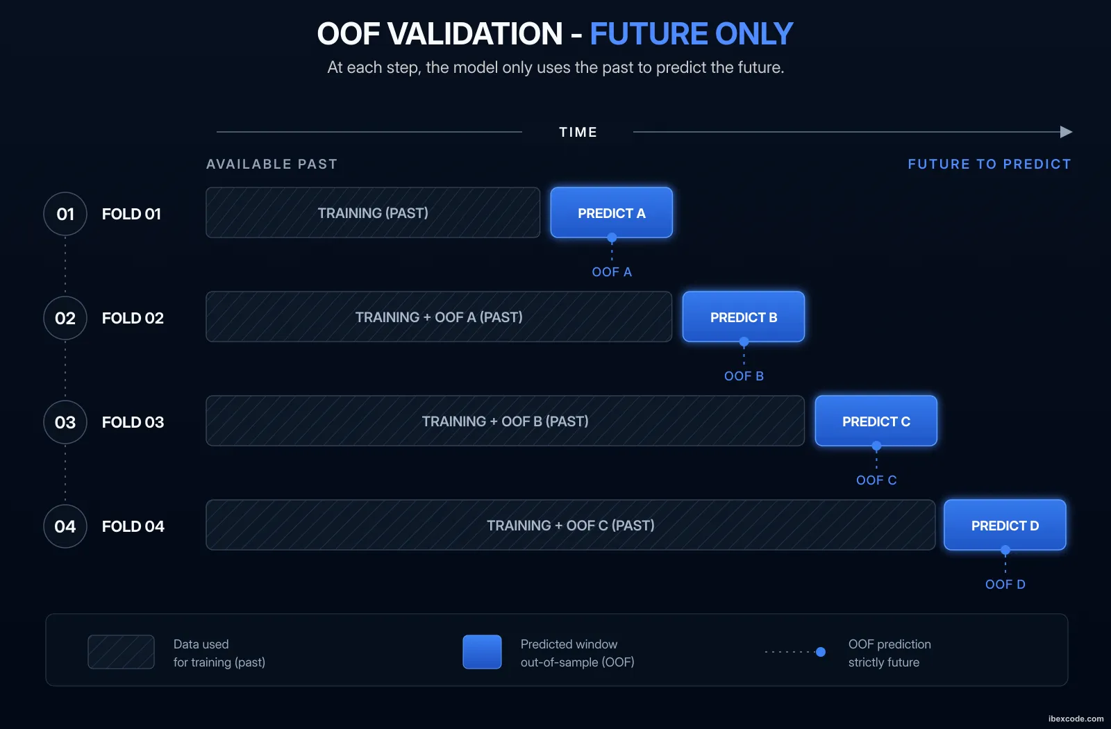
Each window extends the available history without ever crossing the temporal boundary of the period it has to predict.

After concatenation, the result is a dataset where every score corresponds to a genuine, out-of-sample historical prediction:

date       features       prediction_L1
─────────────────────────────────────────
t₁            ...              0.42
t₂            ...              0.71
t₃            ...              0.33
t₄            ...              0.64

These predictions can then become features for the next level without exposing it to predictions produced in-sample.

---

5. The event as the atomic unit of validation

The temporal dimension isn’t the only constraint on the split.

In a ranking problem, observations belonging to the same event aren’t independent. Their position only makes sense relative to the other candidates in the same group.

An event can therefore never be split across multiple folds.

If an event contains:

Event 42
├── A
├── B
├── C
├── D
└── E

its five candidates must all belong to the same segment.

The atomic unit of validation, then, isn’t the dataset row but the entire event.

This property has to be preserved in the OOF folds, in model comparisons, and in any statistical procedures that follow.

It also rules out a subtler form of contamination: letting a model learn part of a group’s context before asking it to rank the group’s remaining observations.

---

6. Causality in feature engineering

Correctly separating the models in time doesn’t, on its own, guarantee the absence of leakage.

Feature engineering has to respect exactly the same causality. For any historical feature computed at time t, the expected property is:

feature(t) = f(observations prior to t)

This constraint applies in particular to:

• Cumulative statistics
• Historical averages
• Frequencies
• Success rates
• Rolling windows
• Category-level aggregations
• Ranking history
• Target-dependent transformations

A single aggregation computed once over the whole dataset before the split can be enough to contaminate every historical observation, even when the models themselves perfectly respect chronology.

The temporal boundary therefore has to be respected starting from the data construction step, not only during model training.

---

7. Isolating learned transformations

The model isn’t the only pipeline component capable of learning from the data.

Some preprocessing steps also estimate parameters from historical data. Normalization, for example, can use the mean and spread observed in the data to transform values:

x' = (x - μ) / σ

where:

• x is the original value
• x' is that same value after normalization
• μ is the mean of the observed values
• σ is their standard deviation, i.e., their spread around that mean

If μ and σ are computed over the whole dataset, they indirectly incorporate information from the future. Historical data then gets transformed using values that weren’t actually available at their own date.

The same risk exists with many other operations:

• filling missing values from observed statistics
• some categorical encodings
• target encoding
• feature selection
• quantile transformations
• dimensionality reduction
• selection based on feature importance
• calibration

The principle, then, is broader than the distinction between model and preprocessing.

The right question is simply:

Does this step learn something from the data in order to do its job?

If it does, the information it relies on has to respect chronology too.

In other words: a preparation step can create temporal leakage exactly like a model can, if it’s built from information that wasn’t yet available at the point in time being considered.

---

8. Recursively propagating the OOF constraint

This property becomes especially important with multiple stacking levels.

Suppose an architecture:

L1 → L2 → L3

L1’s temporal OOF predictions are used to build L2’s dataset.

But then training L2 on the entirety of that dataset and using its in-sample predictions to train L3 would reintroduce exactly the leakage that was eliminated between L1 and L2.

The constraint therefore has to be recursive: every level that feeds a downstream one has to produce its own out-of-sample predictions while preserving temporal causality.

In other words, every boundary between two levels is a new validation boundary.

It’s a structural property of the stack, not a check bolted on after training.

---

9. Stack depth and the erosion of usable history

Strict causality introduces a cost that’s less visible than compute time: part of the history simply can’t be used by downstream levels.

Consider several temporal segments:

A → B → C → D → E

To produce the first level’s OOF predictions:

A       → predict B
A+B     → predict C
A+B+C   → predict D
A+B+C+D → predict E

No genuine future-only OOF prediction can be generated for A, since no earlier period is available.

L2’s dataset therefore necessarily starts later than L1’s. If L2, in turn, has to produce OOF predictions for L3, another portion of the history becomes unavailable.

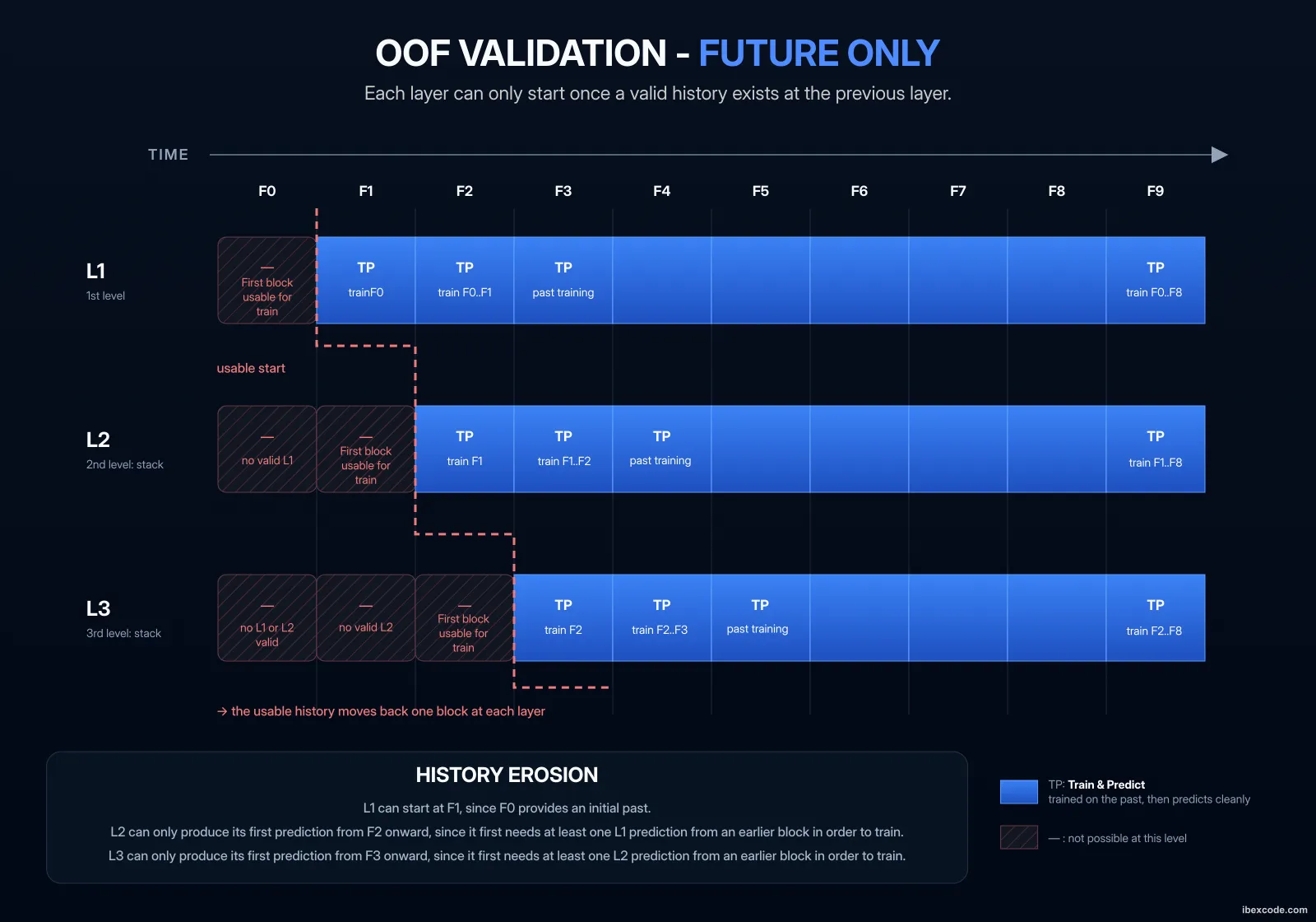
Stack depth therefore creates a trade-off between:

• combination capacity
• available historical depth
• window size
• number of folds
• statistical stability of the later levels

The OOF split, then, isn’t just a validation parameter. It directly shapes the architecture’s design.

---

10. From OOF models to production inference

The models trained while building the temporal folds initially serve one precise purpose: producing the out-of-sample predictions needed to train the downstream levels.

That doesn’t mean they necessarily have to be discarded once the OOF datasets have been built.

Depending on the chosen architecture, several inference strategies are possible. The fold models can be kept and their predictions combined, for instance, or they can be used only to build the OOF dataset, with a separate model trained on a larger history for inference.

In the first case, for a level made up of several temporal folds, this results in something like:

Level
├── fold model 1
├── fold model 2
├── fold model 3
├── ...
└── fold model N

While building the OOF dataset, each model is subject to a strict temporal constraint: it can only produce training predictions for observations that come after its training data.

For a new observation coming after all of these historical periods, though, several of these models can be used simultaneously and their outputs aggregated.

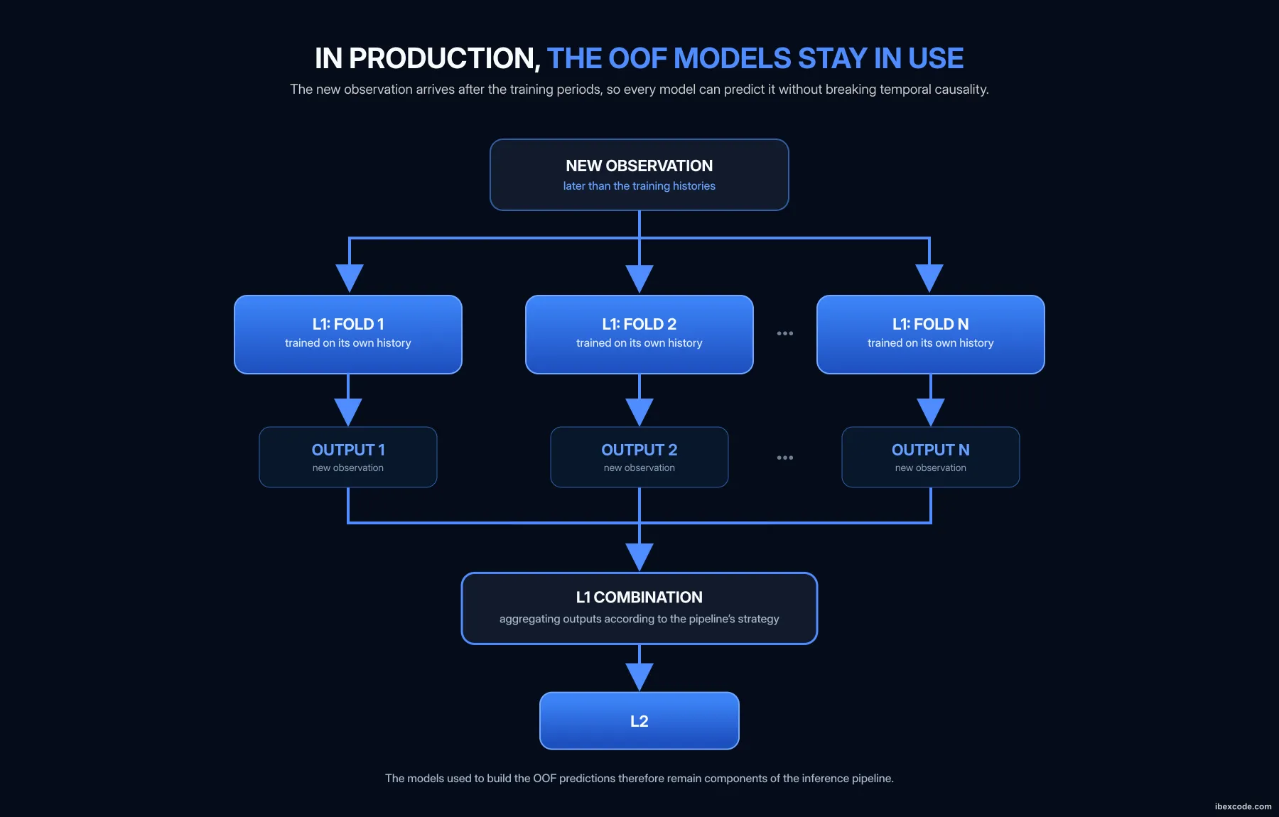
Depending on the strategy chosen, the models used to build the OOF dataset can therefore also become components of the inference pipeline.

One advantage of this choice is that it lets you exploit several models built at different points in the history, rather than always treating folds as purely temporary validation artifacts.

It isn’t, however, a requirement of the OOF method itself.

Another architecture may instead use the folds solely to produce out-of-sample training data, then build the inference model separately.

The important distinction, then, is this:

• OOF generation determines how to build historical predictions without information leakage
• the inference strategy determines which models will actually be used once the system is deployed

These two decisions are related, but they shouldn’t be conflated.

Whatever strategy is chosen, one additional constraint remains: the signals used to train a downstream level must stay representative of what it will actually receive at inference time.

A significant difference between these two situations can introduce a distribution shift, even when temporal causality is perfectly respected.

The absence of data leakage is therefore a necessary condition for the stack’s validity, but it doesn’t remove the need to check consistency between training conditions and production conditions.

---

11. Calibrating models on a dedicated time period

Calibration doesn’t necessarily happen only at the system’s final output.

Whenever a model produces a score that needs a probabilistic interpretation, a calibration step can be attached to it.

Two functions need to be distinguished, then:

• the model, which learns to produce a signal useful for prediction or ranking
• the calibrator, which learns to attach a probability to that signal

Conceptually:

data → model → score → calibrator → probability

Not every component of a multi-level architecture necessarily needs to produce probabilities, though.

Calibration is therefore neither mandatory at every level nor necessarily a single transformation applied at the very end of the stack. It can be attached specifically to the models whose outputs need a probabilistic interpretation.

Calibration depends on the model’s role

In an architecture made up of several models, some signals can be used directly by the next level, while others need calibration first.

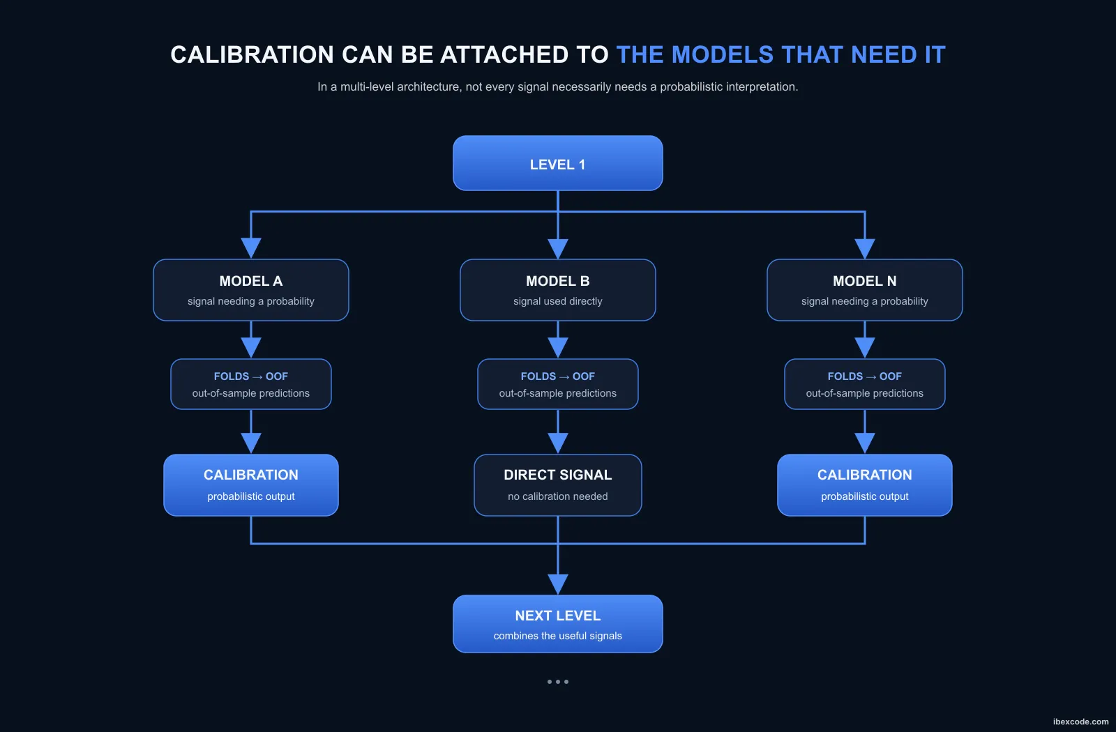
What matters, then, isn’t the number or exact position of the calibrators, but their function:

When necessary, turning the signal produced by a model into a probability with a genuine statistical interpretation.

This distinction also keeps OOF generation and calibration from being conflated. OOF predictions answer an out-of-sample validation constraint; calibration answers a different question: what probability can reasonably be associated with the signal produced by a model?

Why use a dedicated calibration period?

A score produced by a model isn’t necessarily a probability. Two candidates scoring, respectively:

score A = 0.8
score B = 0.4

can be correctly ordered without those values actually meaning an 80% and a 40% probability of occurring.

Calibration is exactly what learns that correspondence between the model’s signal and the frequency actually observed.

For that, it needs two pieces of information:

model prediction + actually observed outcome

The calibrator shouldn’t be fit on in-sample predictions — that is, predictions produced by a model that was trained on those same observations.

The reason is simple: a model generally performs better on the data it was trained on than on new data.

Take a simplified example.

Suppose a certain score level corresponds to:

80% success rate
on the data used to train the model

but

65% success rate
on new observations

A calibration built from the first set of data could end up mapping that score to a probability close to 80%, when its actual behavior on genuinely new observations sits closer to 65%.

The calibrator, then, also learns from data. It has to be fit on out-of-sample predictions, produced on observations the model in question didn’t use to learn.

Several protocols can satisfy this constraint. In the protocol described here, a dedicated time period is set aside for calibration, after the period used to train the model.

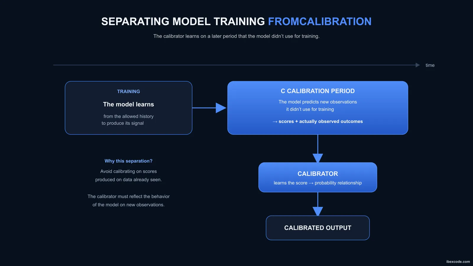
The model is first trained on the historical data available within its training period. It then produces predictions on a later period that was not used for training. It’s these predictions, paired with the actually observed outcomes, that are used to fit the calibrator.

The calibrator therefore learns to interpret the model’s behavior in a situation much closer to the one that actually matters: when it encounters new observations.

So the temporal separation doesn’t just protect model training from data leakage. It also keeps the calibration from being built artificially optimistic.

Calibration has to match the signal actually used

Temporal isolation alone isn’t enough, though.

The calibrator learns a relationship:

model signal → observed probability

The signal used to train it, then, has to stay representative of what it will need to interpret at inference time.

If how that signal is produced changes significantly between calibration and production, the learned relationship may no longer hold in the same way.

A change to the model, its training history, how several outputs are combined, or an upstream transformation can, for example, shift the distribution of scores the calibrator receives.

Two distinct properties therefore have to be preserved:

Calibration must be learned from out-of-sample predictions, produced on observations the model in question didn’t use to learn.

and:

The signal used to learn the calibration must stay representative of what will be produced at inference time.

The first protects against a calibration that looks artificially favorable because it was built from in-sample predictions.

The second protects against a mismatch between the conditions under which the calibrator was fitted and the conditions it will actually be used in.

A learned component in its own right

The calibrator, in the end, has to be treated as a learned component of the system, on the same footing as any other transformation whose parameters are estimated from data.

It has:

• training data
• a temporal boundary
• learned parameters
• a relationship with the signal it transforms
• and usage conditions that have to stay consistent with those of its training

The number and position of the calibrators therefore depend on the role of the different models and the nature of their outputs, not on the structure of the stack itself: nothing requires one calibrator per fold, and nothing rules out a single final calibration for the whole stack either.

The general rule is simpler than that:

Every calibration must be learned on out-of-sample predictions that are representative of the signal it will have to interpret after deployment.

Calibration is therefore one more learning boundary in the system, and it has to be validated with the same rigor as the models it accompanies.

---

12. Reusing the test set and selection bias

Even when no future data ever crosses the pipeline, another source of bias appears once many experiments get compared on the same test period.

This mechanism isn’t data leakage in the strict sense: the model never accesses the test data during training.

The bias comes from experiment selection.

Suppose several dozen variants are evaluated on the same sample:

Model A               → 35.8%
Model B               → 35.9%
New feature           → 36.0%
Model C               → 35.7%
New combination       → 36.1%
...

Each result influences the next decision: keep a feature, abandon an architecture, tweak a hyperparameter, or explore a new combination.

As the number of experiments grows, so does the risk of selecting a configuration that unintentionally exploits the statistical quirks of that specific period, rather than a genuinely generalizable improvement.

That’s why a small gain on the test set, on its own, isn’t treated as sufficient proof.

It has to be considered in light of how many experiments were run, and weighed against other evidence: temporal stability, paired comparison, bootstrap, consistency across different segments, and the behavior of the complete system.

The test set therefore remains an out-of-training measurement, but repeatedly reusing it means small gains have to be treated with caution.

---

13. Statistical robustness of observed gains

A rigorous temporal validation guarantees that models are compared under realistic conditions. It doesn’t, however, guarantee that every observed difference between two models reflects a real improvement.

Suppose two models are evaluated on exactly the same events:

Model A: 35.7%
Model B: 36.1%

Over this period, B is indeed better by 0.4 point.

But another question remains open:

Is B genuinely better, or did we simply evaluate both models over a period that happened to favor it slightly?

Some events favor A, others favor B. When the final gap is small, a handful of events that happen to favor one model can be enough to flip their ranking.

So what has to be measured isn’t just the average gap, but also how stable that gap is.

Comparing models on the same events

Comparisons are done in a paired way: A and B are always evaluated on exactly the same events.

The event, once again, is the indivisible unit of the problem.

A bootstrap procedure can then be used to simulate many alternative samples from the observed period.

The idea is to randomly draw events, with replacement:

Original sample:

[E1, E2, E3, E4, E5, E6, E7, ...]


Some resamples:

Bootstrap 1: [E4, E7, E7, E12, E2, ...]
Bootstrap 2: [E3, E1, E9, E9, E14, ...]
Bootstrap 3: [E8, E2, E4, E4, E11, ...]
...

Some events show up several times, others not at all.

For each of these samples, both models’ performance is recomputed and compared:

Δ = performance(B) - performance(A)

After a large number of repetitions, instead of a single +0.4 point gap, we’re left with a distribution of possible gaps.

Conceptually:

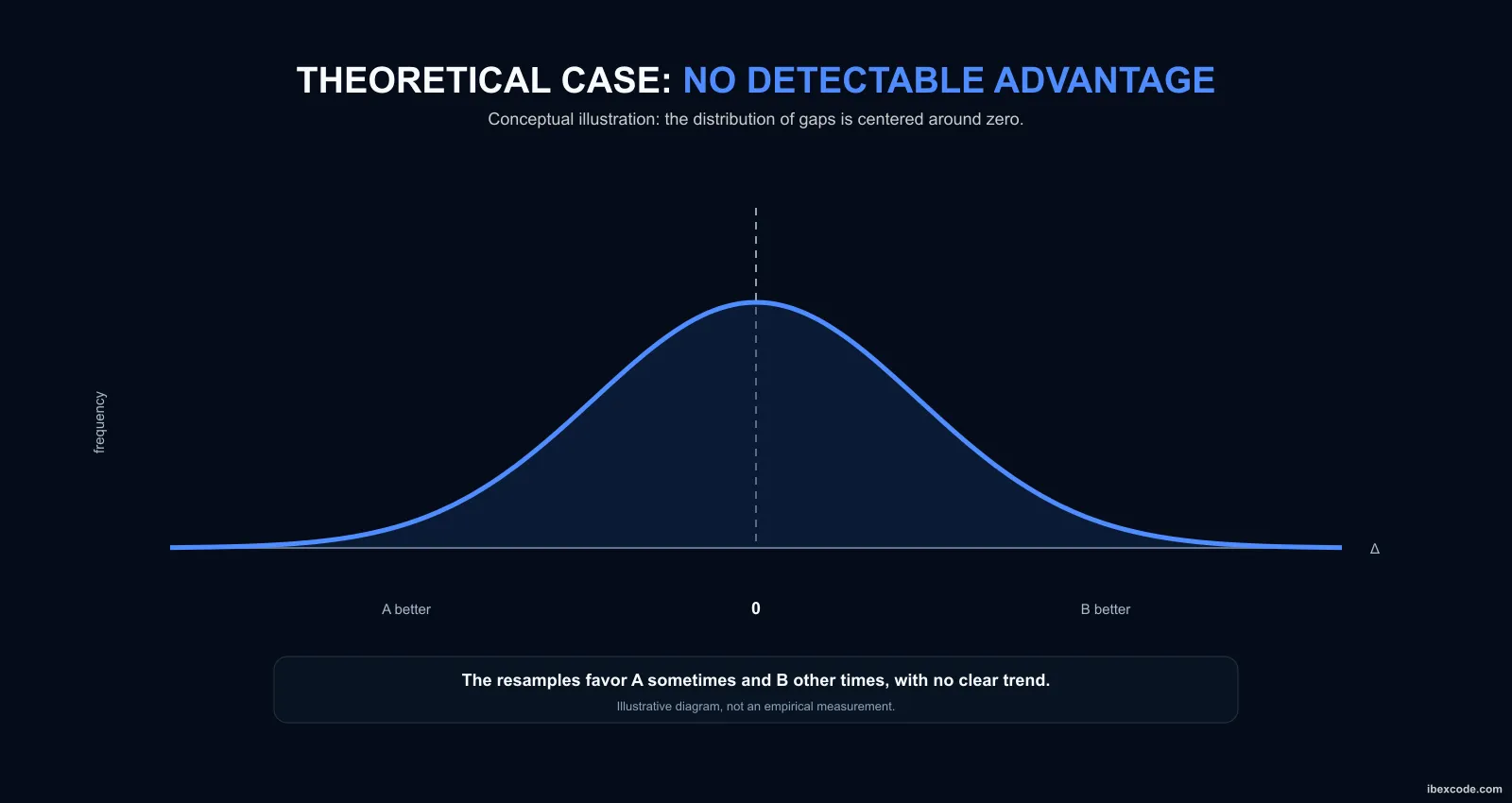
What this distribution lets us check

If B has a robust advantage, the large majority of resamples should keep favoring B:

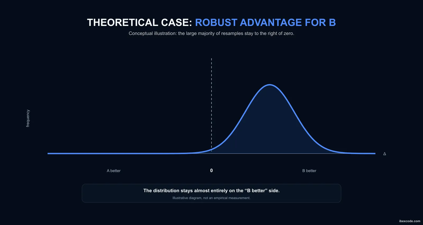
Conversely, if the distribution crosses zero substantially:

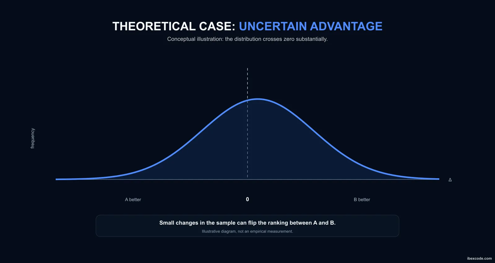
it means that small changes in the sample’s composition are regularly enough to erase B’s advantage, or even make A come out ahead.

The result:

B = 36.1%
A = 35.7%

remains perfectly accurate for the period that was measured.

What the bootstrap calls into question isn’t that measurement — it’s how solid the conclusion drawn from it actually is.

A measured difference isn’t necessarily an exploitable improvement

This distinction matters especially once an architecture is already mature and the gains being sought get smaller.

A new model can achieve a better average metric without the gap being stable enough to justify:

• more complexity
• longer training time
• more expensive inference
• new artifacts to maintain
• or replacing the model currently in production

The decision to promote it, then, doesn’t rest solely on:

metric(B) > metric(A)

but on a more demanding question:

Does the data provide enough evidence to consider the observed advantage robust?

The paired bootstrap is one of the tools used to answer that question.

It complements temporal validation: temporal validation aims to reproduce realistic inference conditions, while the paired bootstrap measures how much the conclusion depends on the particular sample that was observed.

---

14. Evaluating a ranking from several angles

The quality of a ranking system can’t be summed up by a single metric.

Two systems can reach similar overall performance while behaving very differently: one might be especially good at the top positions, while the other more faithfully reproduces the overall ordering of candidates.

Evaluation therefore has to look at several complementary properties.

Quality of the top positions

In many ranking problems, not every position carries the same weight.

A mistake between the top two candidates can have far more consequences than a swap between two candidates near the bottom of the ranking.

Metrics like HitRate@K directly measure the system’s ability to surface the relevant candidates among its top positions.

NDCG@K goes further by accounting for both relevance and position: a correct answer placed very high in the ranking is worth more than the same answer placed lower down.

These metrics answer a targeted question, then:

Does the system place the important candidates high enough in the ranking?

Consistency of the ranking as a whole

Focusing only on the top positions, though, can hide how the rest of the ranking behaves.

Rank-based metrics assess whether the produced order stays broadly consistent with the order actually observed.

A system can therefore be very good at identifying the top candidate while ordering the rest fairly poorly.

Conversely, another system can produce a globally very consistent ranking without being systematically better at the top position.

These two behaviors aren’t equivalent, and a single score cannot adequately describe both.

Quality of the probabilities, when they exist

When a system also produces probabilities, a third property needs evaluating: their calibration.

A probability of 0.8 only genuinely means “80%” if, across a large enough number of comparable situations, the associated event actually occurs about eight times out of ten.

This property can be studied with tools such as:

• the Brier Score
• calibration curves
• comparing predicted probabilities against actually observed frequencies

This is a different dimension from ranking quality.

A system can order the candidates perfectly well while still being overconfident in its probabilities. Conversely, well-calibrated probabilities don’t guarantee that the best candidates are always placed in the right order.

Evaluating properties rather than chasing a universal score

The goal, then, isn’t to find a single metric that summarizes every aspect of the system’s performance.

It’s to check several properties:

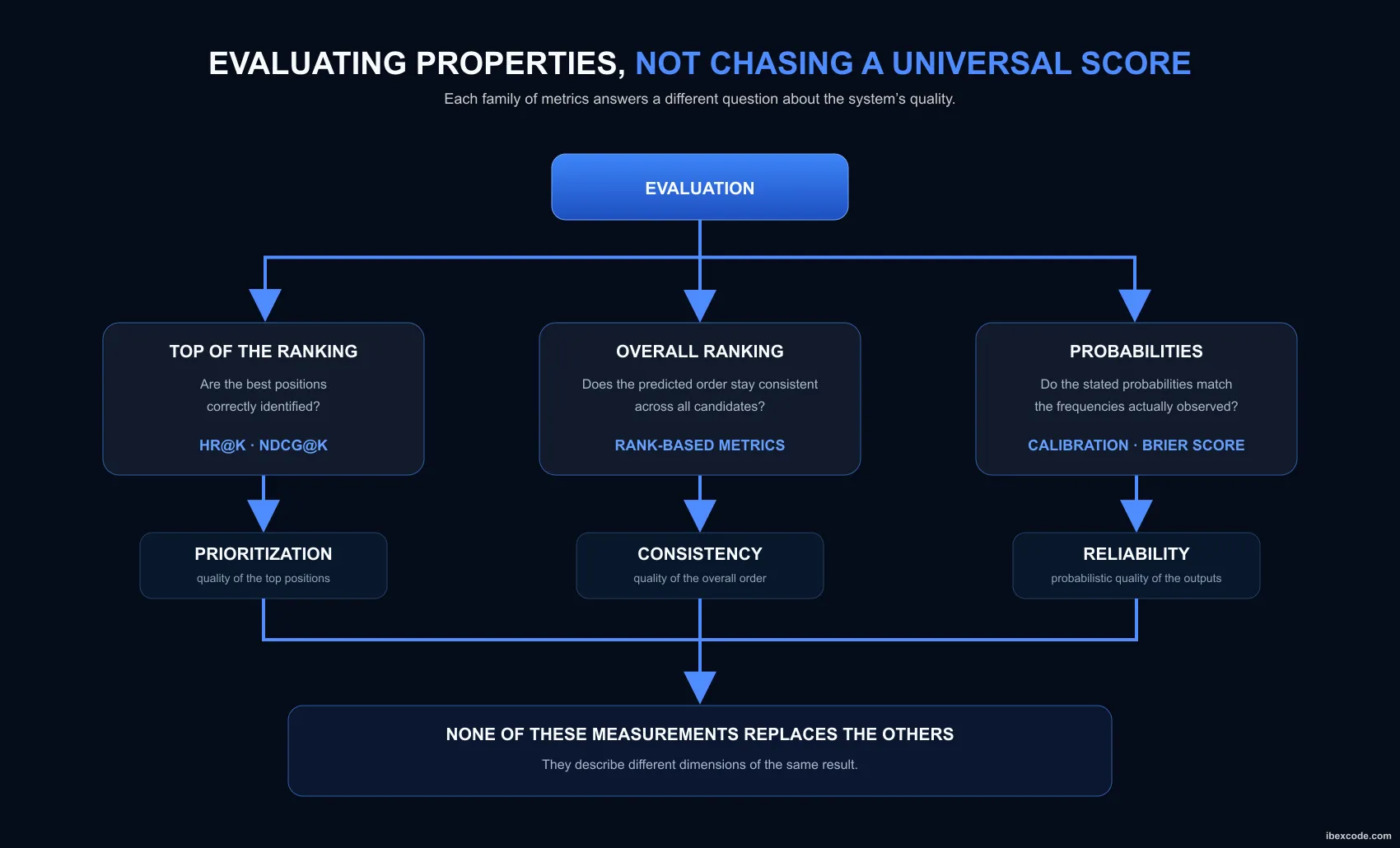
These measurements aren’t competing with each other. They describe different dimensions of the same result.

This approach matters especially when comparing two closely matched configurations. An improvement on one metric can sometimes mask a regression on another.

The comparison, then, has to be driven by the properties the system genuinely needs to preserve, rather than trying to reduce its behavior to a single score.

Evaluating a ranking system is less about asking “what’s its score?” than about determining precisely along which dimensions it’s better, equivalent, or worse than another configuration.

---

15. Computational cost of the protocol

Multi-level temporal validation carries a significant computational cost: a single “model” no longer necessarily corresponds to a single training run.

To produce OOF predictions without temporal leakage, each model has to be trained successively on several historical windows:

A model
    │
    ├── fold 1 training
    ├── fold 2 training
    ├── fold 3 training
    ├── ...
    └── fold N training

This has to be repeated for every model involved and, in a multi-level architecture, for every level that in turn has to produce OOF predictions for the next one.

The overall cost, then, looks more like:

N folds × level-1 models
+
calibrations associated with the level-1 models
+
N folds × level-2 models
+
calibrations associated with the level-2 models
+
N folds × level-k models
+
calibrations associated with the level-k models

or, more compactly:

Σₖ(OOF trainings for level k + calibrations associated with level k)

Calibration isn’t a single operation tacked onto the end of this chain. It’s attached to the models that need it and has its own learning process — in the protocol described here, one built on a dedicated time period.

On top of that comes hyperparameter search. When a configuration has to be evaluated under realistic temporal conditions, a single experiment can therefore require dozens of training runs before it can even be compared to the baseline.

The cost of validation is part of the cost of the model

It would be possible to substantially cut this load by using fewer folds, reusing predictions produced under different conditions, or simplifying some validation steps.

But such an optimization is only worthwhile if it preserves the exact properties the protocol is meant to guarantee.

The trade-off, then, isn’t simply:

more compute ↔ less compute

but rather:

computational cost
        ↕
fidelity of the temporal simulation
        ↕
amount of usable data

The number and size of the folds, for example, simultaneously affect training time, how much history is available to each model, and how many OOF predictions can be passed on to the downstream levels.

These parameters, then, have to be treated as architectural choices, not just as knobs for speeding up or slowing down an experiment.

Research and production don’t carry exactly the same cost

The cost also needs to be considered differently depending on the context.

During research, a new hypothesis can require rebuilding a large part of the chain just to measure its impact under conditions comparable to the baseline.

In production, the artifacts needed for inference have already been built and validated. The computational cost of the validation protocol is therefore mostly incurred during training and experimentation; day-to-day cost then depends on the inference strategy chosen and how many models actually run.

This distinction matters: the computational complexity of an ML system isn’t measured only by the cost of a single production prediction. It also includes the cost of producing an evaluation reliable enough to decide that a new version deserves to be deployed.

---

16. Design principles of the validation protocol

In the end, the architecture rests on a handful of invariants. They aren’t precautions bolted on after training — they directly shape how the datasets, folds, and the stack’s different levels are built.

1. Strict temporal causality Every prediction associated with a given instant t is produced by a model trained exclusively on observations that predate t.

2. Group integrity The event is the indivisible unit of validation. All of its candidates belong to the same temporal segment and the same fold.

3. Causal feature engineering Every historical statistic, aggregation, or data-dependent feature is computed using only the information that would genuinely have been available at the simulated point in time.

4. Stacking exclusively Out-of-Fold No level of the stack is ever trained on predictions produced by a model that has already seen the observations in question. Its inputs are built from OOF predictions that themselves respect temporal causality.

5. Propagating the OOF constraint across levels This property is recursive: whenever one level feeds the next, it in turn has to produce out-of-sample predictions that preserve temporal causality. Every boundary in the stack is therefore a new validation boundary.

6. Isolating every learned transformation Every operation whose parameters are estimated from data respects a temporal boundary suited to its role. Training-related transformations are fit only on the allowed data. Whenever calibration is needed, it’s learned from out-of-sample predictions; in the protocol described here, a later time period is set aside for it.

7. Consistency between OOF construction and production inference The inference strategy can either keep the fold models or use models built specifically for production. Either way, the signals received by the downstream levels have to stay representative of what they were trained on.

8. Accounting for test-set reuse bias The test set remains entirely excluded from model training. Repeatedly consulting it over the course of many experiments can nonetheless introduce a selection bias: a configuration can end up favored by that period’s statistical quirks. Small observed gains are therefore interpreted in light of how many experiments were run and how stable they are.

9. Paired comparisons at the event level Models are compared on exactly the same events. When the gaps are small, their variability is estimated in order to distinguish a sufficiently stable improvement from a difference that could simply be explained by the sample’s particular composition.

10. Promotion based on the robustness of the gain A one-off improvement on a metric isn’t considered sufficient. A new configuration has to keep its advantage across the full temporal protocol, stay consistent on the properties being evaluated, and provide enough benefit to justify any additional complexity or computational cost it introduces.

These invariants have a direct consequence: the validation protocol is part of the system’s architecture.

Changing how historical features are built, how OOF predictions are produced, how temporal boundaries are defined, how models are calibrated, or how validation groups are formed amounts to changing the experiment itself.

The metrics obtained before and after such a change, therefore, aren’t necessarily directly comparable.

---

17. The validation protocol as a component of the architecture

In a multi-level temporal system, a model’s performance can’t be interpreted independently of the protocol that produced it.

Two results are only genuinely comparable if you know, among other things:

• the temporal boundaries used
• the unit used to group the folds
• how the historical features were built
• the training scope of the transformations
• the OOF generation method
• how the OOF predictions propagate between levels
• how calibration is isolated
• how the test period was used
• the uncertainty around the measured gaps

This changes how validation has to be thought about. It’s no longer a step performed after the model is designed — it becomes a constraint that runs through the entire system.

The protocol determines what a historical prediction actually means and, as a result, what each metric is actually measuring.

---

18. Conclusion

For a single, isolated temporal model, avoiding data leakage can be summed up in one simple rule: train on the past, evaluate on the future.

In a ranking system that combines historical feature engineering, several models, stacking, and calibration, that rule can no longer be applied only to the initial data split. It has to be preserved throughout the entire architecture.

Every level that learns, transforms, or passes along information is a new boundary that needs controlling.

The predictions used to build a downstream level must have been produced out-of-sample, with no access to the future. Learned transformations must respect their own temporal scope. Calibrators must be fit on out-of-sample predictions that are representative of inference conditions — in the protocol described here, calibration relies on dedicated time periods for exactly that reason. And finally, both the individual levels and the assembled system have to be evaluated under conditions consistent with how they’ll actually be used.

Behind all these constraints lies the same invariant:

At every simulated instant, the system’s complete state must be reconstructible using only the information that would genuinely have been available at that instant.

This discipline has a cost. Generating OOF predictions multiplies the number of training runs, each additional level shrinks part of the history usable by the next one, calibration introduces its own data and artifacts, and statistical evaluation pushes the experimental cost up further still.

But this complexity isn’t gratuitous: it’s what makes it possible to know what the resulting performance numbers actually measure.

A slightly higher score has little value if the data used to obtain it indirectly contains future information. In the same way, an improvement observed over a given period isn’t necessarily sufficient if it disappears at the smallest change in the sample.

Validation, then, has to answer two complementary questions:

Could the system have produced this prediction using only the information available at that instant?

and:

Is the measured improvement robust enough to be considered genuine progress?

It’s this combination — temporal causality, OOF construction, out-of-sample calibration, and statistical robustness — that turns a sequence of metrics into an evaluation you can actually act on.

In a multi-level temporal ML system, the validation protocol therefore isn’t a procedure applied after the architecture has been designed.

It’s part of it.